Note
Click here to download the full example code
Neural Transfer with PyTorch
Author: Alexis Jacq
Introduction
Welcome! This tutorial explains how to impletment the Neural-Style algorithm developed by Leon A. Gatys, Alexander S. Ecker and Matthias Bethge.
Neural what?
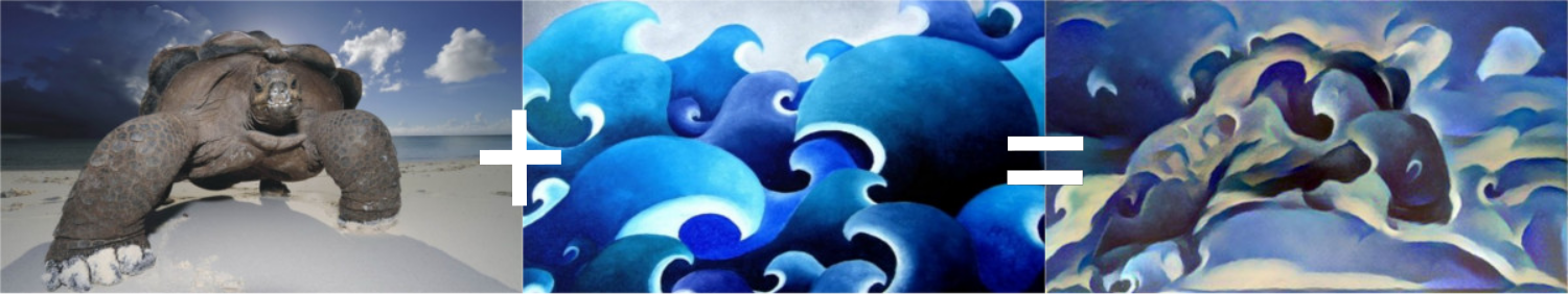
The Neural-Style, or Neural-Transfer, is an algorithm that takes as input a content-image (e.g. a turtle), a style-image (e.g. artistic waves) and return the content of the content-image as if it was ‘painted’ using the artistic style of the style-image:
How does it work?
The principle is simple: we define two distances, one for the content (\(D_C\)) and one for the style (\(D_S\)). \(D_C\) measures how different the content is between two images, while \(D_S\) measures how different the style is between two images. Then, we take a third image, the input, (e.g. a with noise), and we transform it in order to both minimize its content-distance with the content-image and its style-distance with the style-image.
OK. How does it work?
Well, going further requires some mathematics. Let \(C_{nn}\) be a pre-trained deep convolutional neural network and \(X\) be any image. \(C_{nn}(X)\) is the network fed by \(X\) (containing feature maps at all layers). Let \(F_{XL} \in C_{nn}(X)\) be the feature maps at depth layer \(L\), all vectorized and concatenated in one single vector. We simply define the content of \(X\) at layer \(L\) by \(F_{XL}\). Then, if \(Y\) is another image of same the size than \(X\), we define the distance of content at layer \(L\) as follow:
Where \(F_{XL}(i)\) is the \(i^{th}\) element of \(F_{XL}\). The style is a bit less trivial to define. Let \(F_{XL}^k\) with \(k \leq K\) be the vectorized \(k^{th}\) of the \(K\) feature maps at layer \(L\). The style \(G_{XL}\) of \(X\) at layer \(L\) is defined by the Gram produce of all vectorized feature maps \(F_{XL}^k\) with \(k \leq K\). In other words, \(G_{XL}\) is a \(K\)x\(K\) matrix and the element \(G_{XL}(k,l)\) at the \(k^{th}\) line and \(l^{th}\) column of \(G_{XL}\) is the vectorial produce between \(F_{XL}^k\) and \(F_{XL}^l\) :
Where \(F_{XL}^k(i)\) is the \(i^{th}\) element of \(F_{XL}^k\). We can see \(G_{XL}(k,l)\) as a measure of the correlation between feature maps \(k\) and \(l\). In that way, \(G_{XL}\) represents the correlation matrix of feature maps of \(X\) at layer \(L\). Note that the size of \(G_{XL}\) only depends on the number of feature maps, not on the size of \(X\). Then, if \(Y\) is another image of any size, we define the distance of style at layer \(L\) as follow:
In order to minimize in one shot \(D_C(X,C)\) between a variable image \(X\) and target content-image \(C\) and \(D_S(X,S)\) between \(X\) and target style-image \(S\), both computed at several layers , we compute and sum the gradients (derivative with respect to \(X\)) of each distance at each wanted layer:
Where \(L_C\) and \(L_S\) are respectivement the wanted layers (arbitrary stated) of content and style and \(w_{CL_C}\) and \(w_{SL_S}\) the weights (arbitrary stated) associated with the style or the content at each wanted layer. Then, we run a gradient descent over \(X\):
Ok. That’s enough with maths. If you want to go deeper (how to compute the gradients) we encourage you to read the original paper by Leon A. Gatys and AL, where everything is much better and much clearer explained.
For our implementation in PyTorch, we already have everything we need: indeed, with PyTorch, all the gradients are automatically and dynamically computed for you (while you use functions from the library). This is why the implementation of this algorithm becomes very comfortable with PyTorch.
PyTorch implementation
If you are not sure to understand all the mathematics above, you will probably get it by implementing it. If you are discovering PyTorch, we recommend you to first read this Introduction to PyTorch.
Packages
We will have recourse to the following packages:
torch,torch.nn,numpy(indispensables packages for neural networks with PyTorch)torch.optim(efficient gradient descents)PIL,PIL.Image,matplotlib.pyplot(load and display images)torchvision.transforms(treat PIL images and transform into torch tensors)torchvision.models(train or load pre-trained models)copy(to deep copy the models; system package)
from __future__ import print_function

import torch
import torch.nn as nn
import torch.nn.functional as F
import torch.optim as optim

from PIL import Image
import matplotlib.pyplot as plt

import torchvision.transforms as transforms
import torchvision.models as models

import copy
Cuda
If you have a GPU on your computer, it is preferable to run the
algorithm on it, especially if you want to try larger networks (like
VGG). For this, we have torch.cuda.is_available() that returns
True if you computer has an available GPU. Then, we can set the
torch.device that will be used in this script. Then, we will use
the method .to(device) that moves a tensor or a module to the desired
device. When we want to move back this tensor or module to the
CPU (e.g. to use numpy), we can use the .cpu() method.
device = torch.device("cuda" if torch.cuda.is_available() else "cpu")
Load images
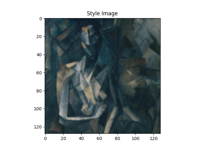
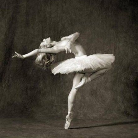
In order to simplify the implementation, let’s start by importing a style and a content image of the same dimentions. We then scale them to the desired output image size (128 or 512 in the example, depending on gpu availablity) and transform them into torch tensors, ready to feed a neural network:
Note
Here are links to download the images required to run the tutorial:
picasso.jpg and
dancing.jpg.
Download these two images and add them to a directory
with name images
# desired size of the output image
imsize = 512 if torch.cuda.is_available() else 128  # use small size if no gpu

loader = transforms.Compose([
    transforms.Resize(imsize),  # scale imported image
    transforms.ToTensor()])  # transform it into a torch tensor


def image_loader(image_name):
    image = Image.open(image_name)
    # fake batch dimension required to fit network's input dimensions
    image = loader(image).unsqueeze(0)
    return image.to(device, torch.float)


style_img = image_loader("images/picasso.jpg")
content_img = image_loader("images/dancing.jpg")

assert style_img.size() == content_img.size(), \
    "we need to import style and content images of the same size"
Imported PIL images have values between 0 and 255. Transformed into torch tensors, their values are between 0 and 1. This is an important detail: neural networks from torch library are trained with 0-1 tensor image. If you try to feed the networks with 0-255 tensor images the activated feature maps will have no sense. This is not the case with pre-trained networks from the Caffe library: they are trained with 0-255 tensor images.
Display images
We will use plt.imshow to display images. So we need to first
reconvert them into PIL images:
unloader = transforms.ToPILImage()  # reconvert into PIL image

plt.ion()

def imshow(tensor, title=None):
    image = tensor.cpu().clone()  # we clone the tensor to not do changes on it
    image = image.squeeze(0)      # remove the fake batch dimension
    image = unloader(image)
    plt.imshow(image)
    if title is not None:
        plt.title(title)
    plt.pause(0.001) # pause a bit so that plots are updated


plt.figure()
imshow(style_img, title='Style Image')

plt.figure()
imshow(content_img, title='Content Image')

Content loss
The content loss is a function that takes as input the feature maps
\(F_{XL}\) at a layer \(L\) in a network fed by \(X\) and
returns the weigthed content distance \(w_{CL}.D_C^L(X,C)\) between
this image and the content image. Hence, the weight \(w_{CL}\) and
the target content \(F_{CL}\) are parameters of the function. We
implement this function as a torch module with a constructor that takes
these parameters as input. The distance \(\|F_{XL} - F_{YL}\|^2\) is
the Mean Square Error between the two sets of feature maps, that can be
computed using a criterion nn.MSELoss stated as a third parameter.
We will add our content losses at each desired layer as additive modules
of the neural network. That way, each time we will feed the network with
an input image \(X\), all the content losses will be computed at the
desired layers and, thanks to autograd, all the gradients will be
computed. For that, we just need to make the forward method of our
module returning the input: the module becomes a ‘’transparent layer’’
of the neural network. The computed loss is saved as a parameter of the
module.
Finally, we define a fake backward method that just calls the
backward method of nn.MSELoss in order to reconstruct the gradient.
This method returns the computed loss: this will be useful when running
the gradient descent in order to display the evolution of style and
content losses.
class ContentLoss(nn.Module):

    def __init__(self, target,):
        super(ContentLoss, self).__init__()
        # we 'detach' the target content from the tree used
        # to dynamically compute the gradient: this is a stated value,
        # not a variable. Otherwise the forward method of the criterion
        # will throw an error.
        self.target = target.detach()

    def forward(self, input):
        self.loss = F.mse_loss(input, self.target)
        return input
Note
Important detail: this module, although it is named ContentLoss,
is not a true PyTorch Loss function. If you want to define your content
loss as a PyTorch Loss, you have to create a PyTorch autograd Function
and to recompute/implement the gradient by the hand in the backward
method.
Style loss
For the style loss, we need first to define a module that compute the gram produce \(G_{XL}\) given the feature maps \(F_{XL}\) of the neural network fed by \(X\), at layer \(L\). Let \(\hat{F}_{XL}\) be the re-shaped version of \(F_{XL}\) into a \(K\)x\(N\) matrix, where \(K\) is the number of feature maps at layer \(L\) and \(N\) the lenght of any vectorized feature map \(F_{XL}^k\). The \(k^{th}\) line of \(\hat{F}_{XL}\) is \(F_{XL}^k\). We let you check that \(\hat{F}_{XL} \cdot \hat{F}_{XL}^T = G_{XL}\). Given that, it becomes easy to implement our module:
def gram_matrix(input):
    a, b, c, d = input.size()  # a=batch size(=1)
    # b=number of feature maps
    # (c,d)=dimensions of a f. map (N=c*d)

    features = input.view(a * b, c * d)  # resise F_XL into \hat F_XL

    G = torch.mm(features, features.t())  # compute the gram product

    # we 'normalize' the values of the gram matrix
    # by dividing by the number of element in each feature maps.
    return G.div(a * b * c * d)
The longer is the feature maps dimension \(N\), the bigger are the values of the Gram matrix. Therefore, if we don’t normalize by \(N\), the loss computed at the first layers (before pooling layers) will have much more importance during the gradient descent. We dont want that, since the most interesting style features are in the deepest layers!
Then, the style loss module is implemented exactly the same way than the content loss module, but it compares the difference in Gram matrices of target and input
class StyleLoss(nn.Module):

    def __init__(self, target_feature):
        super(StyleLoss, self).__init__()
        self.target = gram_matrix(target_feature).detach()

    def forward(self, input):
        G = gram_matrix(input)
        self.loss = F.mse_loss(G, self.target)
        return input
Load the neural network
Now, we have to import a pre-trained neural network. As in the paper, we are going to use a pretrained VGG network with 19 layers (VGG19).
PyTorch’s implementation of VGG is a module divided in two child
Sequential modules: features (containing convolution and pooling
layers) and classifier (containing fully connected layers). We are
just interested by features:
Some layers have different behavior in training and in evaluation. Since we
are using it as a feature extractor. We will use .eval() to set the
network in evaluation mode.
cnn = models.vgg19(pretrained=True).features.to(device).eval()
Additionally, VGG networks are trained on images with each channel normalized by mean=[0.485, 0.456, 0.406] and std=[0.229, 0.224, 0.225]. We will use them to normalize the image before sending into the network.
cnn_normalization_mean = torch.tensor([0.485, 0.456, 0.406]).to(device)
cnn_normalization_std = torch.tensor([0.229, 0.224, 0.225]).to(device)

# create a module to normalize input image so we can easily put it in a
# nn.Sequential
class Normalization(nn.Module):
    def __init__(self, mean, std):
        super(Normalization, self).__init__()
        # .view the mean and std to make them [C x 1 x 1] so that they can
        # directly work with image Tensor of shape [B x C x H x W].
        # B is batch size. C is number of channels. H is height and W is width.
        self.mean = torch.tensor(mean).view(-1, 1, 1)
        self.std = torch.tensor(std).view(-1, 1, 1)

    def forward(self, img):
        # normalize img
        return (img - self.mean) / self.std
A Sequential module contains an ordered list of child modules. For
instance, vgg19.features contains a sequence (Conv2d, ReLU,
MaxPool2d, Conv2d, ReLU…) aligned in the right order of depth. As we
said in Content loss section, we wand to add our style and content
loss modules as additive ‘transparent’ layers in our network, at desired
depths. For that, we construct a new Sequential module, in which we
are going to add modules from vgg19 and our loss modules in the
right order:
# desired depth layers to compute style/content losses :
content_layers_default = ['conv_4']
style_layers_default = ['conv_1', 'conv_2', 'conv_3', 'conv_4', 'conv_5']

def get_style_model_and_losses(cnn, normalization_mean, normalization_std,
                               style_img, content_img,
                               content_layers=content_layers_default,
                               style_layers=style_layers_default):
    cnn = copy.deepcopy(cnn)

    # normalization module
    normalization = Normalization(normalization_mean, normalization_std).to(device)

    # just in order to have an iterable access to or list of content/syle
    # losses
    content_losses = []
    style_losses = []

    # assuming that cnn is a nn.Sequential, so we make a new nn.Sequential
    # to put in modules that are supposed to be activated sequentially
    model = nn.Sequential(normalization)

    i = 0  # increment every time we see a conv
    for layer in cnn.children():
        if isinstance(layer, nn.Conv2d):
            i += 1
            name = 'conv_{}'.format(i)
        elif isinstance(layer, nn.ReLU):
            name = 'relu_{}'.format(i)
            # The in-place version doesn't play very nicely with the ContentLoss
            # and StyleLoss we insert below. So we replace with out-of-place
            # ones here.
            layer = nn.ReLU(inplace=False)
        elif isinstance(layer, nn.MaxPool2d):
            name = 'pool_{}'.format(i)
        elif isinstance(layer, nn.BatchNorm2d):
            name = 'bn_{}'.format(i)
        else:
            raise RuntimeError('Unrecognized layer: {}'.format(layer.__class__.__name__))

        model.add_module(name, layer)

        if name in content_layers:
            # add content loss:
            target = model(content_img).detach()
            content_loss = ContentLoss(target)
            model.add_module("content_loss_{}".format(i), content_loss)
            content_losses.append(content_loss)

        if name in style_layers:
            # add style loss:
            target_feature = model(style_img).detach()
            style_loss = StyleLoss(target_feature)
            model.add_module("style_loss_{}".format(i), style_loss)
            style_losses.append(style_loss)

    # now we trim off the layers after the last content and style losses
    for i in range(len(model) - 1, -1, -1):
        if isinstance(model[i], ContentLoss) or isinstance(model[i], StyleLoss):
            break

    model = model[:(i + 1)]

    return model, style_losses, content_losses
Note
In the paper they recommend to change max pooling layers into average pooling. With AlexNet, that is a small network compared to VGG19 used in the paper, we are not going to see any difference of quality in the result. However, you can use these lines instead if you want to do this substitution:
# avgpool = nn.AvgPool2d(kernel_size=layer.kernel_size,
#                         stride=layer.stride, padding = layer.padding)
# model.add_module(name,avgpool)
Input image
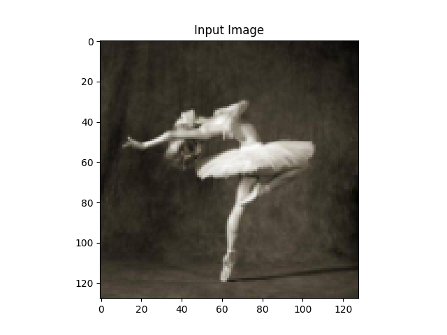
Again, in order to simplify the code, we take an image of the same dimensions than content and style images. This image can be a white noise, or it can also be a copy of the content-image.
input_img = content_img.clone()
# if you want to use a white noise instead uncomment the below line:
# input_img = torch.randn(content_img.data.size(), device=device)

# add the original input image to the figure:
plt.figure()
imshow(input_img, title='Input Image')
Gradient descent
As Leon Gatys, the author of the algorithm, suggested
here,
we will use L-BFGS algorithm to run our gradient descent. Unlike
training a network, we want to train the input image in order to
minimise the content/style losses. We would like to simply create a
PyTorch L-BFGS optimizer optim.LBFGS, passing our image as the
Tensor to optimize. We use .requires_grad_() to make sure that this
image requires gradient.
def get_input_optimizer(input_img):
    # this line to show that input is a parameter that requires a gradient
    optimizer = optim.LBFGS([input_img.requires_grad_()])
    return optimizer
Last step: the loop of gradient descent. At each step, we must feed
the network with the updated input in order to compute the new losses,
we must run the backward methods of each loss to dynamically compute
their gradients and perform the step of gradient descent. The optimizer
requires as argument a “closure”: a function that reevaluates the model
and returns the loss.
However, there’s a small catch. The optimized image may take its values between \(-\infty\) and \(+\infty\) instead of staying between 0 and 1. In other words, the image might be well optimized and have absurd values. In fact, we must perform an optimization under constraints in order to keep having right vaues into our input image. There is a simple solution: at each step, to correct the image to maintain its values into the 0-1 interval.
def run_style_transfer(cnn, normalization_mean, normalization_std,
                       content_img, style_img, input_img, num_steps=300,
                       style_weight=1000000, content_weight=1):
    """Run the style transfer."""
    print('Building the style transfer model..')
    model, style_losses, content_losses = get_style_model_and_losses(cnn,
        normalization_mean, normalization_std, style_img, content_img)
    optimizer = get_input_optimizer(input_img)

    print('Optimizing..')
    run = [0]
    while run[0] <= num_steps:

        def closure():
            # correct the values of updated input image
            input_img.data.clamp_(0, 1)

            optimizer.zero_grad()
            model(input_img)
            style_score = 0
            content_score = 0

            for sl in style_losses:
                style_score += sl.loss
            for cl in content_losses:
                content_score += cl.loss

            style_score *= style_weight
            content_score *= content_weight

            loss = style_score + content_score
            loss.backward()

            run[0] += 1
            if run[0] % 50 == 0:
                print("run {}:".format(run))
                print('Style Loss : {:4f} Content Loss: {:4f}'.format(
                    style_score.item(), content_score.item()))
                print()

            return style_score + content_score

        optimizer.step(closure)

    # a last correction...
    input_img.data.clamp_(0, 1)

    return input_img
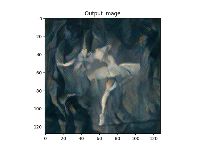
Finally, run the algorithm
output = run_style_transfer(cnn, cnn_normalization_mean, cnn_normalization_std,
                            content_img, style_img, input_img)

plt.figure()
imshow(output, title='Output Image')

# sphinx_gallery_thumbnail_number = 4
plt.ioff()
plt.show()
Out:
Building the style transfer model..
Optimizing..
run [50]:
Style Loss : 113.277611 Content Loss: 18.683996

run [100]:
Style Loss : 34.805576 Content Loss: 17.087635

run [150]:
Style Loss : 14.311416 Content Loss: 15.260895

run [200]:
Style Loss : 7.176407 Content Loss: 13.325481

run [250]:
Style Loss : 4.137866 Content Loss: 11.692221

run [300]:
Style Loss : 2.977307 Content Loss: 10.373799
Total running time of the script: ( 3 minutes 28.364 seconds)