Note
Click here to download the full example code
Spatial Transformer Networks Tutorial
Author: Ghassen HAMROUNI

In this tutorial, you will learn how to augment your network using a visual attention mechanism called spatial transformer networks. You can read more about the spatial transformer networks in the DeepMind paper
Spatial transformer networks are a generalization of differentiable attention to any spatial transformation. Spatial transformer networks (STN for short) allow a neural network to learn how to perform spatial transformations on the input image in order to enhance the geometric invariance of the model. For example, it can crop a region of interest, scale and correct the orientation of an image. It can be a useful mechanism because CNNs are not invariant to rotation and scale and more general affine transformations.
One of the best things about STN is the ability to simply plug it into any existing CNN with very little modification.
# License: BSD
# Author: Ghassen Hamrouni

from __future__ import print_function
import torch
import torch.nn as nn
import torch.nn.functional as F
import torch.optim as optim
import torchvision
from torchvision import datasets, transforms
import matplotlib.pyplot as plt
import numpy as np

plt.ion()   # interactive mode
Loading the data
In this post we experiment with the classic MNIST dataset. Using a standard convolutional network augmented with a spatial transformer network.
device = torch.device("cuda" if torch.cuda.is_available() else "cpu")

# Training dataset
train_loader = torch.utils.data.DataLoader(
    datasets.MNIST(root='.', train=True, download=True,
                   transform=transforms.Compose([
                       transforms.ToTensor(),
                       transforms.Normalize((0.1307,), (0.3081,))
                   ])), batch_size=64, shuffle=True, num_workers=4)
# Test dataset
test_loader = torch.utils.data.DataLoader(
    datasets.MNIST(root='.', train=False, transform=transforms.Compose([
        transforms.ToTensor(),
        transforms.Normalize((0.1307,), (0.3081,))
    ])), batch_size=64, shuffle=True, num_workers=4)
Out:
Downloading http://yann.lecun.com/exdb/mnist/train-images-idx3-ubyte.gz
Downloading http://yann.lecun.com/exdb/mnist/train-labels-idx1-ubyte.gz
Downloading http://yann.lecun.com/exdb/mnist/t10k-images-idx3-ubyte.gz
Downloading http://yann.lecun.com/exdb/mnist/t10k-labels-idx1-ubyte.gz
Processing...
Done!
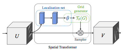
Depicting spatial transformer networks
Spatial transformer networks boils down to three main components :
- The localization network is a regular CNN which regresses the transformation parameters. The transformation is never learned explicitly from this dataset, instead the network learns automatically the spatial transformations that enhances the global accuracy.
- The grid generator generates a grid of coordinates in the input image corresponding to each pixel from the output image.
- The sampler uses the parameters of the transformation and applies it to the input image.
Note
We need the latest version of PyTorch that contains affine_grid and grid_sample modules.
class Net(nn.Module):
    def __init__(self):
        super(Net, self).__init__()
        self.conv1 = nn.Conv2d(1, 10, kernel_size=5)
        self.conv2 = nn.Conv2d(10, 20, kernel_size=5)
        self.conv2_drop = nn.Dropout2d()
        self.fc1 = nn.Linear(320, 50)
        self.fc2 = nn.Linear(50, 10)

        # Spatial transformer localization-network
        self.localization = nn.Sequential(
            nn.Conv2d(1, 8, kernel_size=7),
            nn.MaxPool2d(2, stride=2),
            nn.ReLU(True),
            nn.Conv2d(8, 10, kernel_size=5),
            nn.MaxPool2d(2, stride=2),
            nn.ReLU(True)
        )

        # Regressor for the 3 * 2 affine matrix
        self.fc_loc = nn.Sequential(
            nn.Linear(10 * 3 * 3, 32),
            nn.ReLU(True),
            nn.Linear(32, 3 * 2)
        )

        # Initialize the weights/bias with identity transformation
        self.fc_loc[2].weight.data.zero_()
        self.fc_loc[2].bias.data.copy_(torch.tensor([1, 0, 0, 0, 1, 0], dtype=torch.float))

    # Spatial transformer network forward function
    def stn(self, x):
        xs = self.localization(x)
        xs = xs.view(-1, 10 * 3 * 3)
        theta = self.fc_loc(xs)
        theta = theta.view(-1, 2, 3)

        grid = F.affine_grid(theta, x.size())
        x = F.grid_sample(x, grid)

        return x

    def forward(self, x):
        # transform the input
        x = self.stn(x)

        # Perform the usual forward pass
        x = F.relu(F.max_pool2d(self.conv1(x), 2))
        x = F.relu(F.max_pool2d(self.conv2_drop(self.conv2(x)), 2))
        x = x.view(-1, 320)
        x = F.relu(self.fc1(x))
        x = F.dropout(x, training=self.training)
        x = self.fc2(x)
        return F.log_softmax(x, dim=1)


model = Net().to(device)
Training the model
Now, let’s use the SGD algorithm to train the model. The network is learning the classification task in a supervised way. In the same time the model is learning STN automatically in an end-to-end fashion.
optimizer = optim.SGD(model.parameters(), lr=0.01)


def train(epoch):
    model.train()
    for batch_idx, (data, target) in enumerate(train_loader):
        data, target = data.to(device), target.to(device)

        optimizer.zero_grad()
        output = model(data)
        loss = F.nll_loss(output, target)
        loss.backward()
        optimizer.step()
        if batch_idx % 500 == 0:
            print('Train Epoch: {} [{}/{} ({:.0f}%)]\tLoss: {:.6f}'.format(
                epoch, batch_idx * len(data), len(train_loader.dataset),
                100. * batch_idx / len(train_loader), loss.item()))
#
# A simple test procedure to measure STN the performances on MNIST.
#


def test():
    with torch.no_grad():
        model.eval()
        test_loss = 0
        correct = 0
        for data, target in test_loader:
            data, target = data.to(device), target.to(device)
            output = model(data)

            # sum up batch loss
            test_loss += F.nll_loss(output, target, size_average=False).item()
            # get the index of the max log-probability
            pred = output.max(1, keepdim=True)[1]
            correct += pred.eq(target.view_as(pred)).sum().item()

        test_loss /= len(test_loader.dataset)
        print('\nTest set: Average loss: {:.4f}, Accuracy: {}/{} ({:.0f}%)\n'
              .format(test_loss, correct, len(test_loader.dataset),
                      100. * correct / len(test_loader.dataset)))
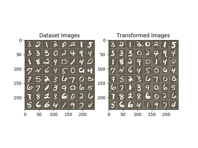
Visualizing the STN results
Now, we will inspect the results of our learned visual attention mechanism.
We define a small helper function in order to visualize the transformations while training.
def convert_image_np(inp):
    """Convert a Tensor to numpy image."""
    inp = inp.numpy().transpose((1, 2, 0))
    mean = np.array([0.485, 0.456, 0.406])
    std = np.array([0.229, 0.224, 0.225])
    inp = std * inp + mean
    inp = np.clip(inp, 0, 1)
    return inp

# We want to visualize the output of the spatial transformers layer
# after the training, we visualize a batch of input images and
# the corresponding transformed batch using STN.


def visualize_stn():
    with torch.no_grad():
        # Get a batch of training data
        data = next(iter(test_loader))[0].to(device)

        input_tensor = data.cpu()
        transformed_input_tensor = model.stn(data).cpu()

        in_grid = convert_image_np(
            torchvision.utils.make_grid(input_tensor))

        out_grid = convert_image_np(
            torchvision.utils.make_grid(transformed_input_tensor))

        # Plot the results side-by-side
        f, axarr = plt.subplots(1, 2)
        axarr[0].imshow(in_grid)
        axarr[0].set_title('Dataset Images')

        axarr[1].imshow(out_grid)
        axarr[1].set_title('Transformed Images')


for epoch in range(1, 20 + 1):
    train(epoch)
    test()

# Visualize the STN transformation on some input batch
visualize_stn()

plt.ioff()
plt.show()
Out:
Train Epoch: 1 [0/60000 (0%)]   Loss: 2.313799
Train Epoch: 1 [32000/60000 (53%)]      Loss: 0.819115

Test set: Average loss: 0.2063, Accuracy: 9431/10000 (94%)

Train Epoch: 2 [0/60000 (0%)]   Loss: 0.381877
Train Epoch: 2 [32000/60000 (53%)]      Loss: 0.342607

Test set: Average loss: 0.1208, Accuracy: 9642/10000 (96%)

Train Epoch: 3 [0/60000 (0%)]   Loss: 0.247812
Train Epoch: 3 [32000/60000 (53%)]      Loss: 0.249339

Test set: Average loss: 0.0961, Accuracy: 9700/10000 (97%)

Train Epoch: 4 [0/60000 (0%)]   Loss: 0.080917
Train Epoch: 4 [32000/60000 (53%)]      Loss: 0.224414

Test set: Average loss: 0.0832, Accuracy: 9754/10000 (98%)

Train Epoch: 5 [0/60000 (0%)]   Loss: 0.204265
Train Epoch: 5 [32000/60000 (53%)]      Loss: 0.142722

Test set: Average loss: 0.0733, Accuracy: 9762/10000 (98%)

Train Epoch: 6 [0/60000 (0%)]   Loss: 0.195066
Train Epoch: 6 [32000/60000 (53%)]      Loss: 0.127173

Test set: Average loss: 0.2049, Accuracy: 9377/10000 (94%)

Train Epoch: 7 [0/60000 (0%)]   Loss: 0.395596
Train Epoch: 7 [32000/60000 (53%)]      Loss: 0.257278

Test set: Average loss: 0.0741, Accuracy: 9772/10000 (98%)

Train Epoch: 8 [0/60000 (0%)]   Loss: 0.051441
Train Epoch: 8 [32000/60000 (53%)]      Loss: 0.182687

Test set: Average loss: 0.0533, Accuracy: 9842/10000 (98%)

Train Epoch: 9 [0/60000 (0%)]   Loss: 0.048953
Train Epoch: 9 [32000/60000 (53%)]      Loss: 0.075130

Test set: Average loss: 0.0634, Accuracy: 9795/10000 (98%)

Train Epoch: 10 [0/60000 (0%)]  Loss: 0.134152
Train Epoch: 10 [32000/60000 (53%)]     Loss: 0.087218

Test set: Average loss: 0.0547, Accuracy: 9833/10000 (98%)

Train Epoch: 11 [0/60000 (0%)]  Loss: 0.099078
Train Epoch: 11 [32000/60000 (53%)]     Loss: 0.169374

Test set: Average loss: 0.0498, Accuracy: 9848/10000 (98%)

Train Epoch: 12 [0/60000 (0%)]  Loss: 0.103957
Train Epoch: 12 [32000/60000 (53%)]     Loss: 0.254779

Test set: Average loss: 0.2090, Accuracy: 9412/10000 (94%)

Train Epoch: 13 [0/60000 (0%)]  Loss: 0.226625
Train Epoch: 13 [32000/60000 (53%)]     Loss: 0.043412

Test set: Average loss: 0.0728, Accuracy: 9784/10000 (98%)

Train Epoch: 14 [0/60000 (0%)]  Loss: 0.273524
Train Epoch: 14 [32000/60000 (53%)]     Loss: 0.200305

Test set: Average loss: 0.0606, Accuracy: 9832/10000 (98%)

Train Epoch: 15 [0/60000 (0%)]  Loss: 0.064689
Train Epoch: 15 [32000/60000 (53%)]     Loss: 0.098237

Test set: Average loss: 0.0502, Accuracy: 9852/10000 (99%)

Train Epoch: 16 [0/60000 (0%)]  Loss: 0.052908
Train Epoch: 16 [32000/60000 (53%)]     Loss: 0.120961

Test set: Average loss: 0.0437, Accuracy: 9863/10000 (99%)

Train Epoch: 17 [0/60000 (0%)]  Loss: 0.078355
Train Epoch: 17 [32000/60000 (53%)]     Loss: 0.093149

Test set: Average loss: 0.0464, Accuracy: 9859/10000 (99%)

Train Epoch: 18 [0/60000 (0%)]  Loss: 0.038080
Train Epoch: 18 [32000/60000 (53%)]     Loss: 0.044862

Test set: Average loss: 0.0519, Accuracy: 9844/10000 (98%)

Train Epoch: 19 [0/60000 (0%)]  Loss: 0.034135
Train Epoch: 19 [32000/60000 (53%)]     Loss: 0.116658

Test set: Average loss: 0.0462, Accuracy: 9866/10000 (99%)

Train Epoch: 20 [0/60000 (0%)]  Loss: 0.048453
Train Epoch: 20 [32000/60000 (53%)]     Loss: 0.114311

Test set: Average loss: 0.0392, Accuracy: 9892/10000 (99%)
Total running time of the script: ( 20 minutes 37.855 seconds)