Transfer Learning tutorial

Author: Sasank Chilamkurthy

In this tutorial, you will learn how to train your network using transfer learning. You can read more about the transfer learning at cs231n notes

Quoting these notes,

In practice, very few people train an entire Convolutional Network from scratch (with random initialization), because it is relatively rare to have a dataset of sufficient size. Instead, it is common to pretrain a ConvNet on a very large dataset (e.g. ImageNet, which contains 1.2 million images with 1000 categories), and then use the ConvNet either as an initialization or a fixed feature extractor for the task of interest.

These two major transfer learning scenarios look as follows:

• Finetuning the convnet: Instead of random initializaion, we initialize the network with a pretrained network, like the one that is trained on imagenet 1000 dataset. Rest of the training looks as usual.
• ConvNet as fixed feature extractor: Here, we will freeze the weights for all of the network except that of the final fully connected layer. This last fully connected layer is replaced with a new one with random weights and only this layer is trained.

# License: BSD
# Author: Sasank Chilamkurthy

from __future__ import print_function, division

import torch
import torch.nn as nn
import torch.optim as optim
from torch.optim import lr_scheduler
import numpy as np
import torchvision
from torchvision import datasets, models, transforms
import matplotlib.pyplot as plt
import time
import os
import copy

plt.ion()   # interactive mode

Load Data

We will use torchvision and torch.utils.data packages for loading the data.

The problem we’re going to solve today is to train a model to classify ants and bees. We have about 120 training images each for ants and bees. There are 75 validation images for each class. Usually, this is a very small dataset to generalize upon, if trained from scratch. Since we are using transfer learning, we should be able to generalize reasonably well.

This dataset is a very small subset of imagenet.

Note

Download the data from here and extract it to the current directory.

# Data augmentation and normalization for training
# Just normalization for validation
data_transforms = {
    'train': transforms.Compose([
        transforms.RandomResizedCrop(224),
        transforms.RandomHorizontalFlip(),
        transforms.ToTensor(),
        transforms.Normalize([0.485, 0.456, 0.406], [0.229, 0.224, 0.225])
    ]),
    'val': transforms.Compose([
        transforms.Resize(256),
        transforms.CenterCrop(224),
        transforms.ToTensor(),
        transforms.Normalize([0.485, 0.456, 0.406], [0.229, 0.224, 0.225])
    ]),
}

data_dir = 'hymenoptera_data'
image_datasets = {x: datasets.ImageFolder(os.path.join(data_dir, x),
                                          data_transforms[x])
                  for x in ['train', 'val']}
dataloaders = {x: torch.utils.data.DataLoader(image_datasets[x], batch_size=4,
                                             shuffle=True, num_workers=4)
              for x in ['train', 'val']}
dataset_sizes = {x: len(image_datasets[x]) for x in ['train', 'val']}
class_names = image_datasets['train'].classes

device = torch.device("cuda:0" if torch.cuda.is_available() else "cpu")

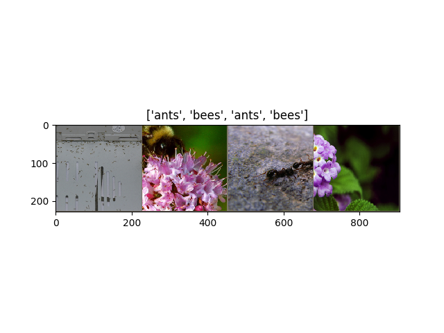
Visualize a few images

Let’s visualize a few training images so as to understand the data augmentations.

def imshow(inp, title=None):
    """Imshow for Tensor."""
    inp = inp.numpy().transpose((1, 2, 0))
    mean = np.array([0.485, 0.456, 0.406])
    std = np.array([0.229, 0.224, 0.225])
    inp = std * inp + mean
    inp = np.clip(inp, 0, 1)
    plt.imshow(inp)
    if title is not None:
        plt.title(title)
    plt.pause(0.001)  # pause a bit so that plots are updated


# Get a batch of training data
inputs, classes = next(iter(dataloaders['train']))

# Make a grid from batch
out = torchvision.utils.make_grid(inputs)

imshow(out, title=[class_names[x] for x in classes])

Training the model

Now, let’s write a general function to train a model. Here, we will illustrate:

• Scheduling the learning rate
• Saving the best model

In the following, parameter scheduler is an LR scheduler object from torch.optim.lr_scheduler.

def train_model(model, criterion, optimizer, scheduler, num_epochs=25):
    since = time.time()

    best_model_wts = copy.deepcopy(model.state_dict())
    best_acc = 0.0

    for epoch in range(num_epochs):
        print('Epoch {}/{}'.format(epoch, num_epochs - 1))
        print('-' * 10)

        # Each epoch has a training and validation phase
        for phase in ['train', 'val']:
            if phase == 'train':
                scheduler.step()
                model.train()  # Set model to training mode
            else:
                model.eval()   # Set model to evaluate mode

            running_loss = 0.0
            running_corrects = 0

            # Iterate over data.
            for inputs, labels in dataloaders[phase]:
                inputs = inputs.to(device)
                labels = labels.to(device)

                # zero the parameter gradients
                optimizer.zero_grad()

                # forward
                # track history if only in train
                with torch.set_grad_enabled(phase == 'train'):
                    outputs = model(inputs)
                    _, preds = torch.max(outputs, 1)
                    loss = criterion(outputs, labels)

                    # backward + optimize only if in training phase
                    if phase == 'train':
                        loss.backward()
                        optimizer.step()

                # statistics
                running_loss += loss.item() * inputs.size(0)
                running_corrects += torch.sum(preds == labels.data)

            epoch_loss = running_loss / dataset_sizes[phase]
            epoch_acc = running_corrects.double() / dataset_sizes[phase]

            print('{} Loss: {:.4f} Acc: {:.4f}'.format(
                phase, epoch_loss, epoch_acc))

            # deep copy the model
            if phase == 'val' and epoch_acc > best_acc:
                best_acc = epoch_acc
                best_model_wts = copy.deepcopy(model.state_dict())

        print()

    time_elapsed = time.time() - since
    print('Training complete in {:.0f}m {:.0f}s'.format(
        time_elapsed // 60, time_elapsed % 60))
    print('Best val Acc: {:4f}'.format(best_acc))

    # load best model weights
    model.load_state_dict(best_model_wts)
    return model

Visualizing the model predictions

Generic function to display predictions for a few images

def visualize_model(model, num_images=6):
    was_training = model.training
    model.eval()
    images_so_far = 0
    fig = plt.figure()

    with torch.no_grad():
        for i, (inputs, labels) in enumerate(dataloaders['val']):
            inputs = inputs.to(device)
            labels = labels.to(device)

            outputs = model(inputs)
            _, preds = torch.max(outputs, 1)

            for j in range(inputs.size()[0]):
                images_so_far += 1
                ax = plt.subplot(num_images//2, 2, images_so_far)
                ax.axis('off')
                ax.set_title('predicted: {}'.format(class_names[preds[j]]))
                imshow(inputs.cpu().data[j])

                if images_so_far == num_images:
                    model.train(mode=was_training)
                    return
        model.train(mode=was_training)

Finetuning the convnet

Load a pretrained model and reset final fully connected layer.

model_ft = models.resnet18(pretrained=True)
num_ftrs = model_ft.fc.in_features
model_ft.fc = nn.Linear(num_ftrs, 2)

model_ft = model_ft.to(device)

criterion = nn.CrossEntropyLoss()

# Observe that all parameters are being optimized
optimizer_ft = optim.SGD(model_ft.parameters(), lr=0.001, momentum=0.9)

# Decay LR by a factor of 0.1 every 7 epochs
exp_lr_scheduler = lr_scheduler.StepLR(optimizer_ft, step_size=7, gamma=0.1)

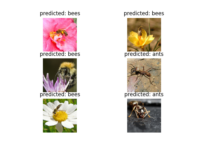
Train and evaluate

It should take around 15-25 min on CPU. On GPU though, it takes less than a minute.

model_ft = train_model(model_ft, criterion, optimizer_ft, exp_lr_scheduler,
                       num_epochs=25)

Out:

Epoch 0/24
----------
train Loss: 0.5119 Acc: 0.7705
val Loss: 0.2494 Acc: 0.9216

Epoch 1/24
----------
train Loss: 0.4073 Acc: 0.8361
val Loss: 0.2335 Acc: 0.9150

Epoch 2/24
----------
train Loss: 0.3775 Acc: 0.8443
val Loss: 0.2279 Acc: 0.9281

Epoch 3/24
----------
train Loss: 0.5218 Acc: 0.7951
val Loss: 0.2613 Acc: 0.9020

Epoch 4/24
----------
train Loss: 0.4783 Acc: 0.7869
val Loss: 0.3122 Acc: 0.9020

Epoch 5/24
----------
train Loss: 0.4914 Acc: 0.7746
val Loss: 0.2654 Acc: 0.9216

Epoch 6/24
----------
train Loss: 0.4815 Acc: 0.8279
val Loss: 0.2956 Acc: 0.9085

Epoch 7/24
----------
train Loss: 0.3547 Acc: 0.8566
val Loss: 0.2662 Acc: 0.9150

Epoch 8/24
----------
train Loss: 0.3241 Acc: 0.8770
val Loss: 0.2552 Acc: 0.9216

Epoch 9/24
----------
train Loss: 0.2853 Acc: 0.8770
val Loss: 0.2434 Acc: 0.9150

Epoch 10/24
----------
train Loss: 0.2662 Acc: 0.9057
val Loss: 0.2494 Acc: 0.9085

Epoch 11/24
----------
train Loss: 0.3991 Acc: 0.8238
val Loss: 0.2500 Acc: 0.9281

Epoch 12/24
----------
train Loss: 0.2888 Acc: 0.8770
val Loss: 0.2269 Acc: 0.9216

Epoch 13/24
----------
train Loss: 0.2602 Acc: 0.9016
val Loss: 0.2200 Acc: 0.9216

Epoch 14/24
----------
train Loss: 0.2599 Acc: 0.8811
val Loss: 0.2138 Acc: 0.9281

Epoch 15/24
----------
train Loss: 0.2988 Acc: 0.8689
val Loss: 0.2228 Acc: 0.9281

Epoch 16/24
----------
train Loss: 0.2522 Acc: 0.8934
val Loss: 0.2213 Acc: 0.9346

Epoch 17/24
----------
train Loss: 0.2866 Acc: 0.8648
val Loss: 0.2153 Acc: 0.9216

Epoch 18/24
----------
train Loss: 0.2613 Acc: 0.8770
val Loss: 0.2155 Acc: 0.9281

Epoch 19/24
----------
train Loss: 0.1685 Acc: 0.9508
val Loss: 0.2171 Acc: 0.9281

Epoch 20/24
----------
train Loss: 0.2950 Acc: 0.8770
val Loss: 0.2065 Acc: 0.9281

Epoch 21/24
----------
train Loss: 0.2537 Acc: 0.8934
val Loss: 0.2229 Acc: 0.9216

Epoch 22/24
----------
train Loss: 0.2344 Acc: 0.8975
val Loss: 0.2228 Acc: 0.9346

Epoch 23/24
----------
train Loss: 0.2462 Acc: 0.9016
val Loss: 0.2210 Acc: 0.9216

Epoch 24/24
----------
train Loss: 0.3504 Acc: 0.8320
val Loss: 0.2131 Acc: 0.9216

Training complete in 28m 41s
Best val Acc: 0.934641

visualize_model(model_ft)

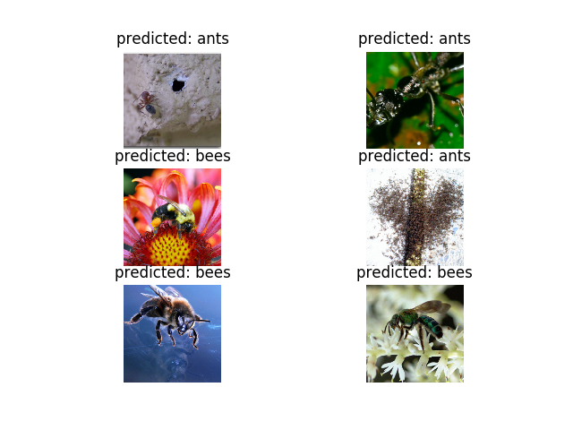
ConvNet as fixed feature extractor

Here, we need to freeze all the network except the final layer. We need to set requires_grad == False to freeze the parameters so that the gradients are not computed in backward().

You can read more about this in the documentation here.

model_conv = torchvision.models.resnet18(pretrained=True)
for param in model_conv.parameters():
    param.requires_grad = False

# Parameters of newly constructed modules have requires_grad=True by default
num_ftrs = model_conv.fc.in_features
model_conv.fc = nn.Linear(num_ftrs, 2)

model_conv = model_conv.to(device)

criterion = nn.CrossEntropyLoss()

# Observe that only parameters of final layer are being optimized as
# opoosed to before.
optimizer_conv = optim.SGD(model_conv.fc.parameters(), lr=0.001, momentum=0.9)

# Decay LR by a factor of 0.1 every 7 epochs
exp_lr_scheduler = lr_scheduler.StepLR(optimizer_conv, step_size=7, gamma=0.1)

Train and evaluate

On CPU this will take about half the time compared to previous scenario. This is expected as gradients don’t need to be computed for most of the network. However, forward does need to be computed.

model_conv = train_model(model_conv, criterion, optimizer_conv,
                         exp_lr_scheduler, num_epochs=25)

Out:

Epoch 0/24
----------
train Loss: 0.5573 Acc: 0.7049
val Loss: 0.2072 Acc: 0.9477

Epoch 1/24
----------
train Loss: 0.5213 Acc: 0.7582
val Loss: 0.2360 Acc: 0.9020

Epoch 2/24
----------
train Loss: 0.5114 Acc: 0.7992
val Loss: 0.2059 Acc: 0.9216

Epoch 3/24
----------
train Loss: 0.3916 Acc: 0.8074
val Loss: 0.2740 Acc: 0.9020

Epoch 4/24
----------
train Loss: 0.3955 Acc: 0.8484
val Loss: 0.1997 Acc: 0.9281

Epoch 5/24
----------
train Loss: 0.3854 Acc: 0.8402
val Loss: 0.2046 Acc: 0.9412

Epoch 6/24
----------
train Loss: 0.3578 Acc: 0.8238
val Loss: 0.2117 Acc: 0.9412

Epoch 7/24
----------
train Loss: 0.3320 Acc: 0.8811
val Loss: 0.2364 Acc: 0.9216

Epoch 8/24
----------
train Loss: 0.3562 Acc: 0.8566
val Loss: 0.2158 Acc: 0.9477

Epoch 9/24
----------
train Loss: 0.3210 Acc: 0.8893
val Loss: 0.2069 Acc: 0.9477

Epoch 10/24
----------
train Loss: 0.4188 Acc: 0.8197
val Loss: 0.2156 Acc: 0.9542

Epoch 11/24
----------
train Loss: 0.3077 Acc: 0.8648
val Loss: 0.2080 Acc: 0.9477

Epoch 12/24
----------
train Loss: 0.2559 Acc: 0.8852
val Loss: 0.2015 Acc: 0.9412

Epoch 13/24
----------
train Loss: 0.3707 Acc: 0.8525
val Loss: 0.2713 Acc: 0.9020

Epoch 14/24
----------
train Loss: 0.3064 Acc: 0.8770
val Loss: 0.2471 Acc: 0.9150

Epoch 15/24
----------
train Loss: 0.3694 Acc: 0.8525
val Loss: 0.2292 Acc: 0.9346

Epoch 16/24
----------
train Loss: 0.3417 Acc: 0.8566
val Loss: 0.2395 Acc: 0.9216

Epoch 17/24
----------
train Loss: 0.2944 Acc: 0.8648
val Loss: 0.2368 Acc: 0.9346

Epoch 18/24
----------
train Loss: 0.4056 Acc: 0.8033
val Loss: 0.2214 Acc: 0.9412

Epoch 19/24
----------
train Loss: 0.3277 Acc: 0.8402
val Loss: 0.2000 Acc: 0.9477

Epoch 20/24
----------
train Loss: 0.3533 Acc: 0.8361
val Loss: 0.2129 Acc: 0.9346

Epoch 21/24
----------
train Loss: 0.3216 Acc: 0.8770
val Loss: 0.2039 Acc: 0.9412

Epoch 22/24
----------
train Loss: 0.3297 Acc: 0.8648
val Loss: 0.2327 Acc: 0.9346

Epoch 23/24
----------
train Loss: 0.2873 Acc: 0.8893
val Loss: 0.2184 Acc: 0.9346

Epoch 24/24
----------
train Loss: 0.2921 Acc: 0.8443
val Loss: 0.2229 Acc: 0.9412

Training complete in 12m 55s
Best val Acc: 0.954248

visualize_model(model_conv)

plt.ioff()
plt.show()

Total running time of the script: ( 41 minutes 51.353 seconds)